MS Excel Secrets - Multi Cell Array Formula
https://ingenuitydias.blogspot.com/2014/03/ms-excel-secrets-multi-cell-array.html
Array formulas are surrounded by curly braces "{ } ". These are added to a formula by pressing the CTRL, SHIFT, and ENTER keys after typing the formula into a cell or cells.
Types of Array Formulas
There are two types of array formulas - those that are located in a single cell of a worksheet (single cell array formula) and those located in multiple cells (multi cell array formula).
Entering the Data
To enter our data into an Excel worksheet as seen in the image.
Types of Array Formulas
There are two types of array formulas - those that are located in a single cell of a worksheet (single cell array formula) and those located in multiple cells (multi cell array formula).
How a Multi Cell Array Formula Works

Read lots more MS Excel Secrets
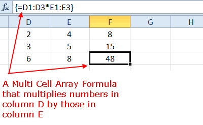
In the image above, the multi cell array formula is located in cells F1:F3 and it carries out the same mathematical operation of multiplication on the data in the ranges of D1:D3 and E1:E3.
Because it is an array formula, each instance or copy of the formula uses different data in its calculations and each instance produces different results.
For example:
The instance of the array formula in cell F1 multiplies the data is cell D1 by the data in cell E1.
The instance of the array formula in cell F2 multiplies the data is cell D2 by the data in cell E2.
The instance of the array formula in cell F3 multiplies the data is cell D3 by the data in cell E3.
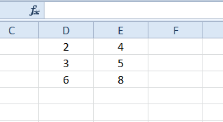
Entering the Data
To enter our data into an Excel worksheet as seen in the image.

Cell Data
D1 - 2
D2 - 3
D3 - 6
E1 - 4
E2 - 5
E3 - 8
Creating the Base Formula
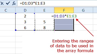
The first step in creating a multi cell array formula is to add the same base formula to all cells where the multi cell array formula will be located.
Creating the Base Formula
The first step in creating a multi cell array formula is to add the same base formula to all cells where the multi cell array formula will be located.

Tutorial Steps
For help with these steps see the image above.
Drag select cells F1 to F3 to highlight them - these are the cells where the multi cell array formula will be located.
Type an equal sign ( = ) on the keyboard to begin the base formula.
Drag select cells D1 to D3 to enter these cell references into the base formula.
Type an asterisk symbol ( * ) on the keyboard since we are multiplying the data in column D by the data in column E.
Drag select cells E1 to E3 to enter these cell references into the base formula.
At this point, leave the worksheet as is - the formula will be completed in the last step of the tutorial when the array formula is created.
Creating the Array Formula
The last step in the tutorial is turning the base formula located in the range F1:F3 into an array formula.
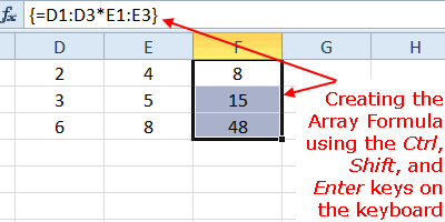
Creating an array formula in Excel is done by pressing the CTRL, SHIFT, and ENTER keys on the keyboard.
Doing so surrounds the formula with curly braces: { } indicating that it is now an array formula.
Tutorial Steps
Hold down the CTRL and SHIFT keys on the keyboard then press and release the ENTERkey to create the array formula.
Release the CTRL and SHIFT keys.
If done correctly, the formulas in cells F1 to F3 will be surrounded by curly braces and each cell will contain a different result as seen in the image above: Cell Result F1 8 - formula multiplies the data in cells D1 * E1 F2 15 - formula multiplies the data in cells D2 * E2 F3 48 - formula multiplies the data in cells D3 * E3
When you click on any of the three cells in the range F1:F3 the completed array formula { = D1:D3 * E1:E3 } appears in the formula bar above the worksheet.
For help with these steps see the image above.
Drag select cells F1 to F3 to highlight them - these are the cells where the multi cell array formula will be located.
Type an equal sign ( = ) on the keyboard to begin the base formula.
Drag select cells D1 to D3 to enter these cell references into the base formula.
Type an asterisk symbol ( * ) on the keyboard since we are multiplying the data in column D by the data in column E.
Drag select cells E1 to E3 to enter these cell references into the base formula.
At this point, leave the worksheet as is - the formula will be completed in the last step of the tutorial when the array formula is created.
Creating the Array Formula
The last step in the tutorial is turning the base formula located in the range F1:F3 into an array formula.

Creating an array formula in Excel is done by pressing the CTRL, SHIFT, and ENTER keys on the keyboard.
Doing so surrounds the formula with curly braces: { } indicating that it is now an array formula.
Tutorial Steps
Hold down the CTRL and SHIFT keys on the keyboard then press and release the ENTERkey to create the array formula.
Release the CTRL and SHIFT keys.
If done correctly, the formulas in cells F1 to F3 will be surrounded by curly braces and each cell will contain a different result as seen in the image above: Cell Result F1 8 - formula multiplies the data in cells D1 * E1 F2 15 - formula multiplies the data in cells D2 * E2 F3 48 - formula multiplies the data in cells D3 * E3
When you click on any of the three cells in the range F1:F3 the completed array formula { = D1:D3 * E1:E3 } appears in the formula bar above the worksheet.


